Hi,
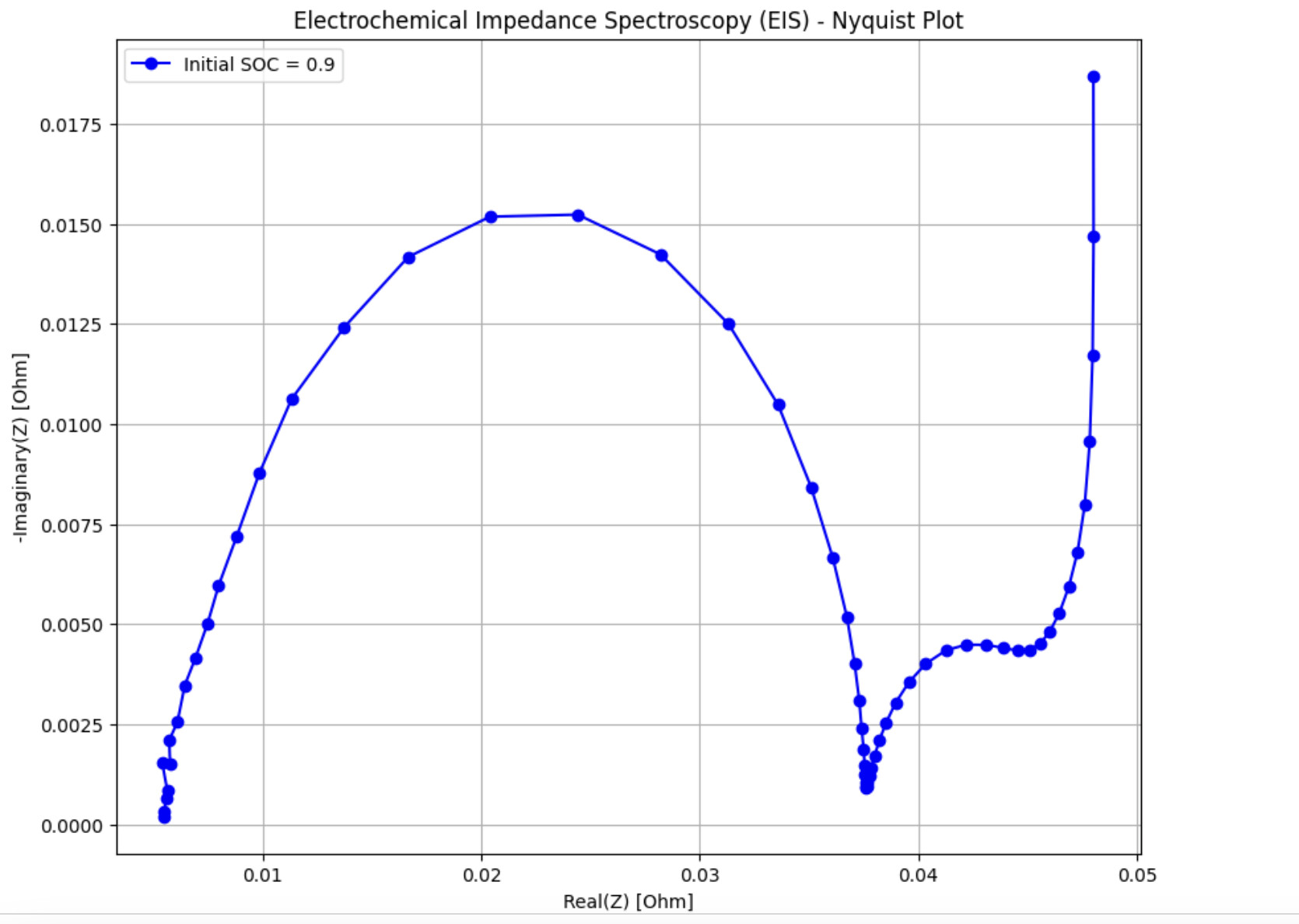
I am trying to obtain EIS from both time domain and pybamm-eis methods, however, the EIS curve is far different from the actual values of resistance 0.025 ohm in the datasheet of LGM50 cell.
Any comment from the PyBaMM team about this.
Thank you for your consideration and looking forward to hearing.
Below is the code I have used for the time domain,
import pybamm
import numpy as np
import matplotlib.pyplot as plt
import time as timer
from scipy.fft import fft
import pandas as pd  # For saving data

# Set up
options = {"thermal": "lumped", "surface form": "differential"}

model = pybamm.lithium_ion.SPMe(options, name="SPMe")
parameter_values = pybamm.ParameterValues("Chen2020")
frequencies = np.logspace(-4, 3, 60)  # Frequency range

# Time domain
I = 50*1e-3  # Current amplitude (100 mA)
number_of_periods = 20
samples_per_period = 16

def current_function(t):
    return I * pybamm.sin(2 * np.pi * pybamm.InputParameter("Frequency [Hz]") * t)

parameter_values["Current function [A]"] = current_function

# SOC values to run
#initial_socs = [0.9, 0.7, 0.5,0.4, 0.3]
initial_socs = [0.9]
colors = ['b', 'g', 'r', 'c', 'm']  # Colors for each SOC

# Initialize a list to store all impedance data
all_data = []

plt.figure(figsize=(10, 8))  # Initialize plot
start_time = timer.time()

for soc, color in zip(initial_socs, colors):
    impedances_time = []
    sim = pybamm.Simulation(
        model, parameter_values=parameter_values, solver=pybamm.ScipySolver()
    )

    for frequency in frequencies:
        # Solve
        period = 1 / frequency
        dt = period / samples_per_period
        t_eval = np.array(range(0, 1 + samples_per_period * number_of_periods)) * dt
        sol = sim.solve(t_eval, inputs={"Frequency [Hz]": frequency}, initial_soc=soc)
        # Extract final two periods of the solution
        time = sol["Time [s]"].entries[-3 * samples_per_period - 1 :]
        current = sol["Current [A]"].entries[-3 * samples_per_period - 1 :]
        voltage = sol["Terminal voltage [V]"].entries[-3 * samples_per_period - 1 :]
        # FFT
        current_fft = fft(current)
        voltage_fft = fft(voltage)
        # Get index of first harmonic
        idx = np.argmax(np.abs(current_fft))
        impedance = -voltage_fft[idx] / current_fft[idx]
        impedances_time.append(impedance)

    # Convert to NumPy array
    impedances_time = np.array(impedances_time)
    # Extract real and imaginary parts
    real_part = np.real(impedances_time)
    imaginary_part = -np.imag(impedances_time)

    # Save data for the current SOC
    soc_data = pd.DataFrame({
        "Frequency [Hz]": frequencies,
        "Real(Z) [Ohm]": real_part,
        "Imaginary(Z) [Ohm]": imaginary_part,
        "SOC": soc
    })
    all_data.append(soc_data)

    # Plot for the current SOC
    plt.plot(real_part, imaginary_part, marker='o', linestyle='-', color=color, label=f"Initial SOC = {soc}")

# Combine all SOC data and save to a single file
all_data_combined = pd.concat(all_data, ignore_index=True)
all_data_combined.to_csv("impedance_data_all_soc_0.1.csv", index=False)

end_time = timer.time()
time_elapsed = end_time - start_time
print("Time domain method: ", time_elapsed, "s")

# Plot settings
plt.title("Electrochemical Impedance Spectroscopy (EIS) - Nyquist Plot")
plt.xlabel("Real(Z) [Ohm]")
plt.ylabel("-Imaginary(Z) [Ohm]")
plt.legend()
plt.grid(True)
plt.show()